Chapter 1: Computation
Before we understand anything about quantum computation, let’s motivate why it might be useful. But what does useful even mean? And so, we begin our journey in the world of theoretical computer science.
Computation? How hard could it be?
We are all intimately familiar with ‘computers’, but perhaps less universal is the concept of ‘computation’. The average person uses their computer to browse the internet, send emails, and look at TikTok. Quantum computers will not displace classical computers for any of those tasks*. We will instead scope our discussion to solving specifically defined mathematical problems. While some of these problems are totally abstract, others are extremely practical. Many of the applications of conventional computers we find so useful are undergirded by these numerical problems: Cryptography protects our data; machine learning algorithms shape the content we see; linear algebra is the key to performing simulations of physical phenomena.
Understandably, we may want to know how ‘difficult’ a problem is for a computer (classical or quantum) to solve. Computer scientists have come up with a concept, known as computational complexity, which categorizes certain problems based on how many resources (whether they be time, operations, or memory) they take to solve.
Let’s take addition as an example. Say I have two numbers, each represented with n bits*. Using a classical computer, I can add those numbers with approximately 9n operations (technically we would call them gates, but let’s just think of them as steps in a recipe)*. As anyone who’s taken a computer science class will know, we can represent the computational intensity of this task with what’s called big-O notation: addition has linear complexity and thus is in $O(n)$. Essentially, this metric codifies that as n increases, the computational overhead required to perform this task (add two n-bit numbers) scales linearly with $n$. However, this need not be the case.
There are problems with constant complexity – $O(1)$. Say we want to know if a $n$-bit number is even or odd. A computer can check this by simply looking at the value of the last bit of the number: If it’s a one, the number is odd; if it’s a zero, the number is even. This holds if n is equal to one or equal to ten million. Thus, we can solve this problem in constant time.
There are problems with higher than linear complexity. Some problems have polynomial complexity, such as $O(n^2)$ or $O(n^3)$. For instance, multiplying two matrices requires polynomial time*. This is much less desirable than a linear complexity, because adding more bits to the problem can substantially increase how long it takes to run. However, many problems are even worse than this and have exponential complexity, like $O(2^n)$. The quintessential example of this is factoring. Given a large integer, it is very time-consuming to break it up into its constituent factors. This forms the basis for modern encryption, which uses the difficult nature of factoring to provide security for encoded data.
Generally, we make a distinction between tasks with polynomial complexity and those with exponential complexity. Anything with polynomial or below complexity is deemed efficient, i.e., tractable for classical computers to solve. Problems with exponential complexity are considered to scale so poorly that they cannot easily be solved using classical computers. This tends to be a useful practical distinction, but it’s worth examining it a bit deeper. Depending on the value of n, an algorithm with $O(n^8)$ (nominally an efficient polynomial algorithm) may be significantly slower than an inefficient exponential $O(1.25^n)$ approach. However, as $n$ tends toward infinity, the polynomial algorithm will eventually win out. Thus, it’s important to consider what the specific complexity is for a given algorithm and use case. Nevertheless, it tends to be the case that in most real applications, we desire polynomial-time, efficient algorithms.
Theoretical computer scientists have a hobby of using complexity to sort problems into different classes. If a problem can be solved in polynomial time, they say it is in class P. Perhaps the most famous problem in computer science relates to class P and another class, NP. NP is the class of problems that can be verified in polynomial time. A problem like factoring is very much in NP – if an algorithm spits out a factor, we can easily check if it’s right by dividing the input by the output. The famous problem asks: is P equal to NP? That is, if I can verify a problem efficiently, can I also compute it efficiently?
Most people think that P is not equal to NP. This intuitively makes sense. If it were possible to efficiently factor large primes, modern encryption schemes wouldn’t be very secure (and lots of resources have been spent trying to figure out how to factor large primes efficiently).
A logical next step, especially given the context of this work, is asking if a quantum computer can solve problems efficiently that a classical computer cannot. We will discuss this further below, but let’s assume for a moment that quantum computers can do the same operations classical computers can (i.e., we can use them like a classical computer, and not access their ‘quantumness’). Because of this, quantum computers can solve problems in the same number of steps as their classical brethren. Thus, the class of problems quantum computers can solve efficiently at least is equal to P.
It turns out that quantum computers can also do some problems efficiently that classical computers can’t. As such, the theorists have defined a separate class from P called ‘BQP’ which includes all problems that can be solved by quantum computers in polynomial time with bounded error. Why bounded error? We will learn that quantum computers are, at their core, probabilistic devices. We will soon examine some algorithms where there is a probability of outputting the wrong result. Luckily, these algorithms typically can achieve higher accuracy via running in longer but still polynomial time. Practically, BQP is the direct quantum analogue to P.
There are several kinds of interesting and potentially practically useful algorithms that are in BQP but not in P*. Notably, factoring can be done in polynomial time on a quantum computer, as can certain kinds of algorithms that relate to chemical simulation. This is really exciting, and is the fundamental reason why the world is interested in developing quantum computers. We will explore this efficient factoring algorithm later in this chapter, and consider other real-world applications in Chapter 4.
But this is no free lunch! As we will examine in Chapter 2, quantum computers are likely to operate slower and with less usable (qu)bits than their classical brethren. Algorithms with equivalent computational complexity are likely to run longer (and require more resources) on a quantum computer than on a classical one. After all, I can readily access billions of transistors operating at multi-GHz speeds on my laptop – that’s pretty good! For a theoretical quantum speedup to result in a practically realizable speedup, it’s likely that the quantum algorithm must reduce an exponential-time problem into a polynomial-time one.
We are now armed with a core motivating principle: quantum computers may be able to solve certain problems faster than classical computers. This is the singular driving force behind the billions of dollars of investment and hundreds of years of person-hours spent on quantum computer development. But we are still hopelessly confused as to what quantum computation is.
A Qubit
Claude Shannon invented the term ‘bit’ in 1948 to refer to units of information*. The term has become a foundational concept for computing. A singular bit can be 0 or 1, and we can encode $2^N$ values in $N$ bits (3 bits gives us $2^3 = 8$ codewords: 000; 001; 010; 011; 100; 101; 110; 111). We can do math on these bits, and use groups of them to encode integers, decimal numbers, sounds, pictures, or video.
Functionally, we implement bits as being voltage levels stored on semiconductor chips. Think of this as banks of light switches, which can either be turned on or off. A row of 5 alternating switches could be in the state 11010, encoding the number 26 in binary ($1*(2^4) + 1*(2^3) + 0*(2^2) + 1*(2^1) + 0*(2^0) = 16 + 8 + 2 = 26$).
We can also do computation on those bits – the simplest operation we can do is flipping an individual bit. Say we flip the last switch in the previous example, transforming its state to 11011. Now, the switches represent a binary 27*. The act of flipping a bit is called a NOT gate. The NOT gate is an example of a 1-bit gate (with one input and output). This logic is codified in its truth table, shown in Table 1. We can also implement a 2-bit gate, such as the AND gate, which takes two bits as inputs and outputs a single bit. That output is 1 if and only if both inputs are also 1 (if A is true AND B is true, then output triue), as shown in Table 2. There are several 2-bit gates, such as AND, OR, XOR (exclusive or), and NAND (not and).
| Input | NOT(Input) |
|---|---|
| 0 | 1 |
| 1 | 0 |
| Input 1 | Input 2 | AND(Input 1, Input 2) |
|---|---|---|
| 0 | 0 | 0 |
| 0 | 1 | 0 |
| 1 | 0 | 0 |
| 1 | 1 | 1 |
It’s now time to begin our first foray into the world of quantum computing. To those most interested in physical implementations, this text’s singular focus on theory for this first section may be disappointing, but the tight interrelation between theory, software, and hardware in the quantum world makes this extremely critical material to understand. So don’t skip it (at least skim it)!
The quantum computing analogue to a bit is a quantum bit, or qubit (incredible creativity in nomenclature). The qubit has several interesting and unique properties, the first and foremost that it can exist in a superposition of states. Pop science articles will typically describe this by saying that the qubit can be both 0 and 1 at the same time. Somehow, this both over- and under-sells the unique properties of the qubit.
It is more accurate to say that a single qubit exists in a probability distribution of states. We are going to use a helpful visual aid known as the Bloch sphere, shown in Fig. 1. This is a 3D unit sphere with an arrow (a vector) pointing to somewhere on the surface of the sphere, shown below. The vertical axis corresponds to states totally analogous to the conventional bit – if the arrow points straight up, we call that the $\ket{0}$ state, and straight down, the $\ket{1}$ state. If we start in $\ket{0}$ and rotate the arrow 180 degrees, we end up in $\ket{1}$ – that’s equivalent to a NOT gate. This operation is shown in Fig. 1B. So far, this is actually exactly the same as conventional bits! Give me 5 qubits, and I can encode 26 in binary via the state $\ket{1} \otimes \ket{1} \otimes \ket{0} \otimes \ket{1} \otimes \ket{0}$. Of course, this would be a tremendous waste of the engineering effort required to give me those qubits, but it does reveal a powerful result: A quantum computer can at least do everything a classical computer can do.
Quantum people use ‘bra ket notation’ to denote quantum states. We’re not going to worry too much about the details here. Just know that if it’s inside $|$these funny lines$\rangle$, it’s a qubit state. $\ket{\psi}$ is a generic variable used to denote an arbitrary qubit state. If we have multiple qubits, we can put them together like so: $\ket{A} \otimes \ket{B}$ or $\ket{AB}$ are equivalent.
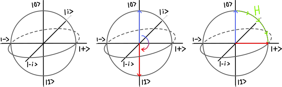
OK, let’s go one step further. What if instead of rotating the arrow by 180 degrees, we rotate it by 90 degrees, towards the horizontal axis – the state labeled $\ket{+}$? This is shown in Fig. 1C. Well, we can now describe the state of the qubit, which we will call $\ket{\psi}$, as being a linear combination of $\ket{0}$ and $\ket{1}$. We will refer to this combination as a superposition. In fact, it is exactly 50% $\ket{0}$ and 50% $\ket{1}$. This should immediately seem strange to you. After all, we would never describe a conventional bit as being half 0 and half 1. The unintuitive and unique property here is that when we measure the qubit, it collapses to either $\ket{0}$ or $\ket{1}$, each with 50% probability*. Crucially, until we measure it, the qubit is still in that superposition: the act of measurement collapses its state. We can express this mathematically like so:
$$ \ket{\psi} = \ket{+} = \frac{1}{\sqrt{2}}\ket{0} + \frac{1}{\sqrt{2}}\ket{1} $$The coefficients in front of $\ket{0}$ and $\ket{1}$ are not the probabilities of measuring each state but are instead ‘amplitudes’. We can translate this amplitude into a probability of measuring each state by squaring it ($1/\sqrt{2}^2 = 1/2$, or 50%). Amplitudes, unlike probabilities, can be negative and complex (have imaginary numbers in them*).
Thus, the state of a single qubit can be described using four continuous parameters (the real and imaginary components of each the two amplitudes). When we draw a vector in a Bloch sphere, we are implicitly projecting this four dimensional vector space down into three dimensions. We can do so without loss of information because the qubit occupies a limited space in those four dimensions: we know that the probabilities of measuring each state must sum to 1! This then creates a restriction on what values the amplitudes can take on. As we describe multiple qubits, we will need even more parameters to characterize the system, expanding into what is known as a multi-dimensional ‘Hilbert space’.
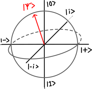
We could also rotate the arrow to a new point on the Bloch sphere called $\ket{\psi'}$, shown in Fig. 2. Note that $\ket{\psi'}$ is much closer to $\ket{0}$ than $\ket{1}$. Correspondingly, if we were to measure $\ket{\psi'}$, it is much more likely to ‘collapse’ to the $\ket{0}$ state than the $\ket{1}$ state. This is the core of the concept of superposition.
There’s a complexity here that I’m glossing over. $\ket{+}$ is a state where the probabilities of measuring $\ket{0}$ and $\ket{1}$ are equal; but it is not the only state where this is true. All points on the circle highlighted in green in Fig. 3, including the states $\ket{-}$, $\ket{i}$, and $\ket{-i}$, have equal probabilities of measuring $\ket{0}$ and $\ket{1}$.
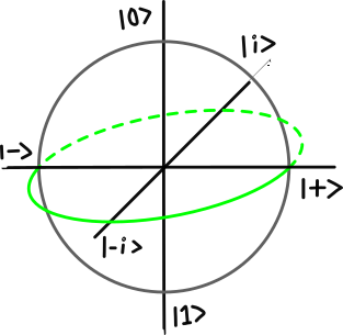
However, these states are not equivalent. We say they have different phases. We can represent these states as linear combinations of the $\ket{0}$ and $\ket{1}$ states:
$$\ket{+} = \frac{1}{\sqrt{2}}\ket{0} + \frac{1}{\sqrt{2}}\ket{1}$$ $$\ket{-} = \frac{1}{\sqrt{2}} \ket{0} - \frac{1}{\sqrt{2}}\ket{1}$$It’s easy to see that the amplitudes of the $\ket{-}$ state have the same magnitudes, but different signs than the amplitudes of $\ket{+}$. While they are impossible to differentiate by a simple measurement in the $\ket{0}$/$\ket{1}$ (computational) basis*, these qubits will behave differently in multi-qubit interactions. As we will see, a critical part of quantum algorithms is how these amplitudes will either constructively or destructively interfere to get the desired results.
Quantum Amplitudes & Probabilities
Quantum amplitudes are essentially what would happen if probabilities could be negative*. Each amplitude in a 2-qubit quantum state like:
$$\ket{\psi} = a\ket{00} + b\ket{01} + c\ket{10} + d\ket{11}$$Corresponds to the probability of measuring that particular outcome. Hence:
$$P(\ket{00}) = |a|^2$$ $$P(\ket{01}) = |b|^2$$ $$P(\ket{10}) = |c|^2$$ $$P(\ket{11}) = |d|^2$$Importantly, $|a|^2+|b|^2+|c|^2+|d|^2$ must equal 1, because those are all the possible options post-measurement. Notice that even if a is negative or complex, the probability of measuring $\ket{00}$ is still positive. This is what we refer to as ‘phase’. As noted above, two qubits could be in different states, but still have the same measurement probabilities, due to a phase difference. Those negative signs are incredibly important to implementing quantum computation, because they allow operations to create constructive and destructive interference. We will see examples of this shortly.
Let’s also revisit the concept of gates. I noted before that with a bit, the only 1-bit gate we can perform is flipping it (AKA the NOT gate). In the qubit example, that NOT gate is equivalent to performing a 180 degree rotation around the sphere. But note that we can also make any arbitrary rotation around the unit sphere! I can go from $\ket{0}$ to $\ket{\psi}$ (that’s a gate) or from $\ket{\psi}$ to $\ket{\psi'}$ (that’s another gate). We can string gates together, and these will also be gates. As we will learn, we can assemble any arbitrary logical operation we want from a more limited set of gates. This is advantageous because certain physical implementations of quantum computing only allow the use of certain gates (or, by their nature, make it easy to use some gates but not others).
Single Qubit Gates are 2x2 Unitary Matrices
All quantum math can be expressed in terms of linear algebra and matrices. We can express qubit states as vectors and 1 qubit gates as 2x2 unitary matrices. A unitary matrix $U$ has the following property: $UU^* = I$, that is, when multiplied by its conjugate transpose, gives the identity matrix. Let’s give an example, using the Hadamard gate, H:
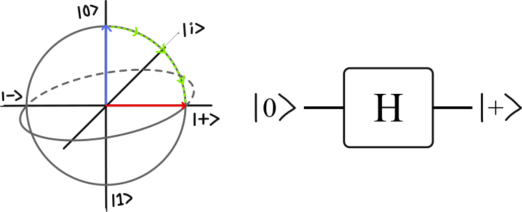
$$\ket{0} = \begin{bmatrix} 1 \\ 0 \end{bmatrix} \hspace{1cm} \ket{1} = \begin{bmatrix} 0 \\ 1 \end{bmatrix}$$ $$ H = \frac{1}{\sqrt{2}} \begin{bmatrix} 1 & 1 \\ 1 & -1 \end{bmatrix} $$ $$ H\ket{0} = \frac{1}{\sqrt[]{2}} \begin{bmatrix} 1*1 + 1*0 \\ 1*1 + 0*-1 \end{bmatrix} = \frac{1}{\sqrt[]{2}} \begin{bmatrix} 1 \\ 1 \end{bmatrix} = \frac{1}{\sqrt[]{2}} (\ket{0} + \ket{1}) = \ket{+} $$You’ll often see circuit diagrams of computations like the below. In these diagrams, each horizontal line represents a single qubit, and each box represents a gate. Gates must always have the same number of inputs and outputs (unlike classical computing, where something like a AND gate has two inputs and one output). The qubit moves left to right in time, experiencing gates along the way. See Fig. 4, where a Hadamard gate (H) transforms an input from the $\ket{0}$ state to the $\ket{+}$ state.
Common 1-Qubit Gates
Here are several of the most common 1 qubit gates. X, Y, and Z all rotate the state 180 degrees around their respective axes. X functions as a bit flip, Z as a phase flip, and Y as a combination of the two. These three are known as Pauli gates. The S and T gates are essentially fractional phase rotations, functioning as 90 and 45 degree rotations respectively. The T gate is particularly important because it is necessary to achieve universal quantum computing in many implementations, but difficult to practically implement. More on that later.
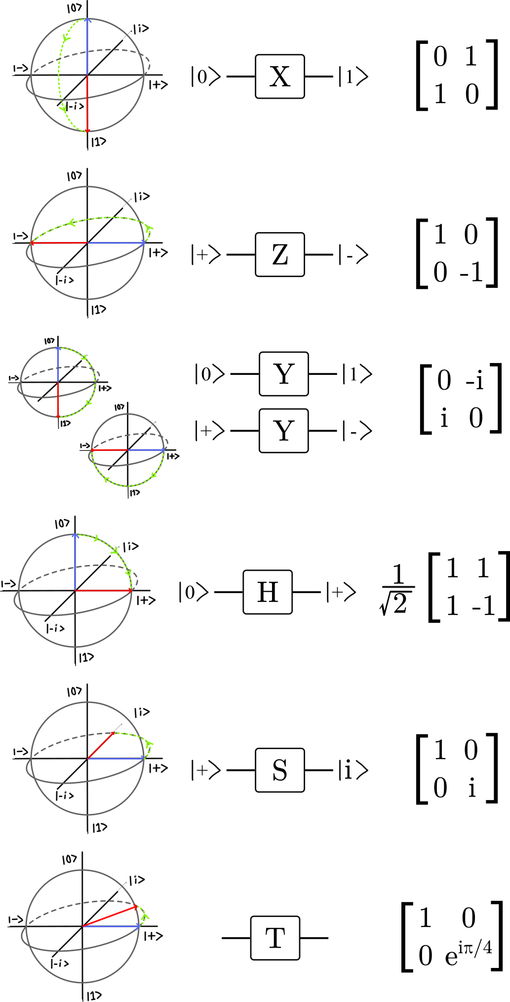
A Diversion into Analog Computing
It’s tempting to read the above and think that a qubit on its own is more powerful than a bit. After all, a bit can be either 0 or 1, but the qubit can encode something in this continuous multi-dimensional vector space! There are a few complications to this. The first is that while we can put the qubit in an arbitrary state, we can only measure it once, which collapses it to either $\ket{0}$ or $\ket{1}$. If given a qubit in a special state, $\ket{\psi} = \alpha \ket{0} + \beta \ket{1}$, we cannot extract the values of $\alpha$ and $\beta$. After all, as soon as you measure the qubit, it will collapse to one of two states and some information will be lost. As a result, it is not possible to encode arbitrarily large amounts of information in a single qubit*. This is dictated by Holevo’s theorem.
Putting that issue aside, there are also problems with the idea of simply using the qubit as an outright analog computer. Analog computing is a very old idea that aims to use continuous values in computation, rather than the discrete values that traditional bits provide. We can visualize this by imagining a special analog water computer. This special computer would be programmed to pump water between several tanks before depositing a specific amount into an output vessel. The volume of the output would correspond to the answer to the question posed to the computer. This is a very attractive idea, and proponents of this kind of computation often argue that it could be substantially more efficient than traditional computing*.
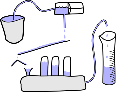
However, analog computing suffers from several difficulties, the primary one being errors in the system. In a traditional computer, every computation can be executed with virtually 100% accuracy. We can do thousands or millions of operations in a row, and get the right answer in the end, because binary operations on our bits are extremely reliable. However, in an analog computer, individual components or gates may not be as precise as desired, and errors may compound over the course of a calculation. Say one of my pumping operations (essentially equivalent to a gate) dispenses 1% more water than it needs to during every individual operation. If that ‘gate’ gets used hundreds of times over a long calculation, the result could be extremely wrong. Moreover, it may be unverifiably wrong! This is a simple but potentially fatal problem for the idea.
As a result, when we talk about quantum computing, we are most often not talking about using it in a ‘analog fashion’. That is – in most algorithms we expect to encode inputs in binary, and get back answers in binary. However, quantum algorithms will put qubits in many intermediate, superimposed states before they return their final answer. Along the way, they will use algorithms that leverage quantum properties to perform active error correction on those qubits, mitigating the build-up of these errors. Quantum computing is thus distinct from both classical binary computing and classical analog computing.
It is worth noting that some in the field are working on ‘quantum simulators’, which is in fact akin to an analog quantum computer. These simulators aim to recreate some sort of quantum mechanical system or property using more macro-scale particles (atoms are commonly used). This kind of simulator is actually what Feynman discussed in his seminal proposal of quantum computation. This approach is distinct from the gate-based quantum computers we’ve been talking about, since it never deals with any sort of digital values. Instead, analog measurements are taken within the simulator, which then correspond to some physical property of the simulated problem. This approach is being actively pursued by many academic groups for problems such as superconductivity. We will further discuss using quantum computers for simulation in sections below, but note that this analog approach is an alternative – one that may be easier and more practical for certain types of problems.
Qubits, plural
So far, we’ve learned that qubits have the property of superposition, wherein they obey probabilistic laws that determine the outcome of any measurement. Let us now examine another unique property of qubits: Entanglement. We are going to talk about entanglement right now as a purely mathematical concept, as something that changes the mathematical representation of the state of the qubit system. It is also a physical phenomenon, one that can be generated using clever engineering on real quantum computing hardware, but let’s put that aside. For now, entanglement is simply a math operation that will enable very unique (and potentially useful) methods of computation.
Put simply, two qubits are entangled when one’s state is dependent on the other’s. Measurement of one qubit affects the state of its entangled counterparts. The prototypical example of this is the two-qubit state $\ket{\psi} = \frac{1}{\sqrt{2}}\ket{00} + \frac{1}{\sqrt{2}}\ket{11}$. If the first qubit is measured to be $\ket{0}$, the state of the second qubit must also be $\ket{0}$. Correspondingly, if we measure one qubit to be $\ket{1}$, the other must also be in state $\ket{1}$. This particular state is known as one of the Bell states*.
Entangled vs. Product States
Some multi-qubit states are entangled, and others are not – these are called product states. Product states can be factored into products of component qubits, while entangled states cannot. For example:
$$\ket{\psi} = \alpha\ket{00} + \beta\ket{01} + \gamma\ket{10} + \delta\ket{11}$$If we can extricate two different single qubit states from this state, then it is a product state:
$$\ket{\psi} =(a\ket{0} + b\ket{1}) \otimes (c\ket{0} + d\ket{1}) = \ket{A} \otimes \ket{B} = \ket{A}\ket{B}$$However, some states cannot be factored like this, such as the example given in the text above:
$$\ket{\psi} = 1/\sqrt{2} \ket{00} + 1/\sqrt{2} \ket{11}$$It’s impossible to factor this into two independent qubit states! These two qubits are maximally entangled. It’s also now impossible to draw them as two independent Bloch spheres.
This should not appear intuitive to the reader. This is not a process implemented with logic gates; it’s not the same as “if qubit A is $\ket{0}$, then qubit B becomes $\ket{0}$.” Instead, it is a quantum mechanical phenomenon. Two qubits can become entangled, then separated, and when one is measured the other’s state will collapse instantaneously. Einstein famously called this ‘spooky action at a distance.’ This property freaked Einstein out a lot, because he understood physics at a very deep level. As someone who doesn’t understand physics that well, I don’t get that worked up about it.
Unfortunately it’s not easy to visualize entanglement, and we have to abandon our trusty friend the Bloch sphere. Originally, each qubit existed in what’s called $\mathbb{C}^2$, where its state was defined by two complex numbers (its amplitudes). We could graph on our 3-dimensional Bloch sphere. A set of N qubits will be in $\mathbb{C}^{2^N}$, and be defined by $2^N$ amplitudes (each a complex number). If the qubits are independent, we could draw the system using N Bloch spheres. However, if these qubits become entangled, their states become dependent on one another, and we no longer can graph the entire system state in any reasonable way. We can and will project this multidimensional vector space down to two or three dimensions, but that’s not helpful for the moment. The crucial thing to understand is that entanglement turns individual qubits into a complex, interdependent system.
Entanglement is a very important enabling property for quantum computation, as we will see. But how does one actually entangle two qubits? Well, we need a way for two qubits to interact. As you might guess, this is done via ‘two-qubit gates’.
There are a variety of two-qubit gates, but one of the most common is CNOT. CNOT, or ‘controlled not,’ is a gate that flips the second qubit (the target) if the first qubit (the control) is $\ket{1}$. Like so:
$$CNOT\ket{11} = \ket{10}$$ $$CNOT\ket{10} = \ket{11}$$ $$CNOT\ket{01} = \ket{01}$$ $$CNOT\ket{00} = \ket{00}$$Crucially, we can apply CNOT to superpositions! Recall that $\ket{+}$ is equal to $1/\sqrt{2} \ket{0} + 1/\sqrt{2} \ket{1}$.
$$CNOT\ket{+}\ket{0} = CNOT(1/\sqrt{2} \ket{00} + 1/\sqrt{2} \ket{10}) = 1/\sqrt{2} \ket{00} + 1/\sqrt{2} \ket{11}$$And now we’ve produced an entangled state! Hooray! We can also draw CNOT gates in our circuit diagram like so:
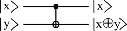
Here’s an important note: Even though $\ket{x}$ is the ‘control’ qubit and $\ket{y}$ is the ‘target’ qubit, $\ket{x}$ is changed by the CNOT gate. This is known as ‘phase kickback’ and we will see more examples of it in the future.
Phase Kickback
Phase kickback is not intuitive at all, so here’s a basic example of the phenomenon:
$$CNOT(\ket{+}\ket{-}) = CNOT(\frac{1}{\sqrt{2}} (\ket{0} + \ket{1}) \otimes \frac{1}{\sqrt{2} } (\ket{0} - \ket{1}) ) $$ $$ =CNOT( \frac{1}{2}\ket{00} - \frac{1}{2}\ket{01} + \frac{1}{2}\ket{10} - \frac{1}{2}\ket{11} ) $$ $$ =\frac{1}{2}\ket{00} - \frac{1}{2}\ket{01} + \frac{1}{2}\ket{11} - \frac{1}{2}\ket{10} $$ $$ =\frac{1}{2}\ket{00} - \frac{1}{2}\ket{01} - \frac{1}{2}\ket{10} + \frac{1}{2}\ket{11} $$ $$ =\frac{1}{\sqrt{2}} (\ket{0} - \ket{1}) \otimes \frac{1}{\sqrt{2}} (\ket{0} - \ket{1}) $$ $$ = \ket{-}\ket{-} $$So our CNOT ended up changing our control qubit, but left the target qubit unchanged. How very strange things are in quantum land!
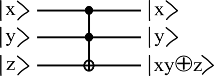
There are also other multi-qubit gates we may want to implement. One oft discussed one is the Toffoli gate, which uses three qubits. People often use Toffolis as short hand for how complex a circuit is – as in “Yeah we can implement that with a thousand qubits and a million Toffolis”. A Toffoli gate is closely related to CNOT and can in fact just be thought of as a CCNOT, or controlled CNOT: $CCNOT\ket{110} = \ket{111}$. A Toffoli has two control qubits and one target qubit. The target qubit’s state is only flipped if both control qubits are $\ket{1}$ (or, as we discussed before, if they are superpositions of $\ket{1}$). The circuit diagram for a Toffoli is below.
Common Multi-Qubit Gates
Here’s a table of common multi-qubit gates and their associated matrices. Note that any gate can be turned into a controlled gate, here denoted by the ‘CU’ gate, where U represents any arbitrary 1-qubit gate.
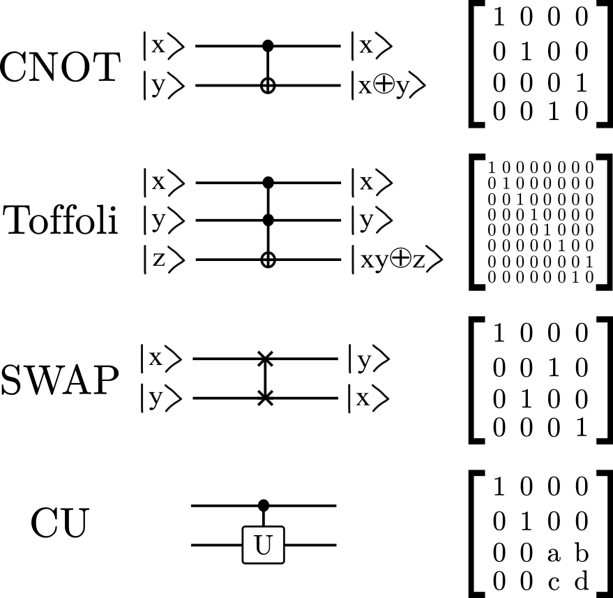
As previously mentioned, depending on the physical implementation of the qubits, some of these gates may be easier or harder to achieve in practice. As a result, it is necessary to ask which of these gates are necessary for quantum computation. A set of gates which can perform all quantum computations is known as a ‘universal gate set’. In classical computing, the NAND gate is a universal gate set all by itself, hence why digital logic is implemented with NAND gates. In quantum computing, we are not so lucky to have a single universal gate. A universal gate set must be able to A) create superposition; B) create entanglement; C) reach complex amplitudes*. One such gate set is {CNOT, H, T}. We shall return to these concepts later in Chapter 2.
It may not be immediately obvious what all this entanglement and qubit business actually enables. One simple and close-enough-to-true way to look at it is by thinking about how much information is embedded inside a multi-bit versus multi-qubit system. In a three-bit system, we can encode $2^3 = 8$ different values. We counted those states out above. In a three-qubit system, we describe the state of the system with 8 complex amplitudes, like so:
$$\ket{\psi} = a\ket{000} + b\ket{001} + c\ket{010} + d\ket{011} + e\ket{100} + f\ket{101} + g\ket{110} + h\ket{111} $$Let me emphasize this: each of these amplitudes (a through h) are complex numbers that would require several bytes to properly represent (potentially many bytes depending on how precise our quantum computation needs to be). The number of these amplitudes scales like $2^N$ with N qubits. That becomes very large, very fast. Note that we cannot arbitrarily access the values of those amplitudes, we can only selectively measure the qubits and collapse the system into a particular state. Nevertheless, we can do intermediate operations that take advantage of the large number of these amplitudes, as well as their ability to constructively and destructively interfere, to perform computations. This is the powerful and unique thing about qubits and quantum computation.
Pure vs. Mixed States
Here’s a very sophisticated piece of quantum terminology (using it will surely give you lots of quantum street cred). All the quantum states we’ve discussed so far are known as ‘pure states’. A pure state is one where we are certain of the quantum state the system is in. It might be a superposition, and measurement outcomes are probabilistic, but the state is known. However, sometimes systems are in unknown or ‘less known’ quantum states. Perhaps we think there’s a 50% chance of a system being in $\ket{\psi}$ and a 50% chance of being in $\ket{\chi}$. We’d characterize this as being in a mixed state.
Pure states are represented by points on the Bloch sphere, as we’ve seen. Mixed states are represented by points inside of the Bloch sphere. The closer a point is to the surface, the more certain we are of the state – i.e. the ‘purer’ it is.
Importantly, mixed states obey the laws of classical probability, not quantum laws. We can accurately say that the system has X% probability of being in a state, without worrying about complex numbers or amplitudes.
We’re now going to look at three different quantum algorithms, in increasing order of complexity. Unfortunately, even the first and simplest quantum algorithm is still non-trivial to understand (so please don’t feel disheartened if you are confused!). The point of looking at these sections is not to beat an understanding of quantum computer science theory into you, but to help you understand the general approaches and unique characteristics of quantum algorithms. So while our examples will grow more complicated as we progress, our analysis will also begin to focus more on high-level takeaways than quantum circuits. Depending on your level of interest, you may want to skim or skip this section, although I do think that understanding generally what a quantum algorithm is can be helpful for thinking about a quantum computer more broadly. On the other hand, if you find yourself actively wishing for more rigor and math, I suggest looking at Thomas Wong’s excellent “Introduction to Classical and Quantum Computing.”
Quantum Advantage: Deutsch-Jozsa Algorithm
Let us examine a simple algorithm that provably improves on what a classical computer can do. But before we do that, we need to get one last piece of preamble out of the way. Those pesky theoretical computer scientists, never happy to make things too simple, often use ‘oracles’ in their problems and algorithms. An oracle is a fancy way of saying a black boxed function that the algorithm in question has access to. The algorithm can call on the oracle as needed and will get back the oracle’s answer. We never worry about the implementation of the oracle, and simply count how many times we need to call upon it. This oracle may not be possible to implement in the real world – or it may take longer computational time than the rest of the algorithm! Nevertheless, the oracle is a helpful tool in the toolbox for theorists to begin their work. Shor’s factoring algorithm began as an oracle implementation, then was fully implemented sans-oracle. In the next two examples, we will use oracles. Both the classical and quantum algorithms will have access to the oracle, but as we will see, the quantum algorithm can successfully solve the problem with fewer calls to that function. This is the most rudimentary kind of distinction between computational classes, known as an oracle separation.
In quantum land, we can both query and receive qubits in superposition. We can represent the oracle in our quantum circuit notation as a multi-qubit gate, like below:
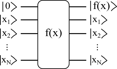
Note that the oracle has n input qubits, and an answer qubit. In standard form, the answer qubit is changed by the oracle’s internal logic, and the input qubit is not. However, for the algorithm we are about to look at, we need to add yet another complication – a phase oracle. This is closely related to the concept of phase kickback, which we discussed above in the context of the CNOT gate. The idea here is that by putting the answer qubit in a particular state ($\ket{-}$) prior to feeding it to the oracle, the oracle operates differently: it instead changes the phase of the input qubits (leaving the answer qubit in that $\ket{-}$ state). There are some mathematics that make this work , but for the purposes of this text, it’s simply another way of defining the black box function, so we will gloss over it. See the below diagram for an example of a phase oracle.
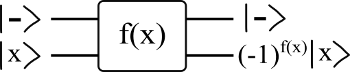
Now, after much deliberation, we can begin looking at the Deutsch-Jozsa algorithm – baby’s first quantum advantage. The problem is contrived and the speedup is not particularly impressive, but it exists nonetheless. The problem is this: You are given an oracle (we will call it $f(x)$), that takes in a bitstring of length n, and outputs either 1 or 0. We know that $f(x)$ has a special property; it is either `constant' or `balanced'. If it is constant, no matter what the input is, it will always output the same value (but we don’t know if that value will be always 0 or always 1). If it is balanced, it will output 0 for exactly half of all input bitstrings, and 1 for the other half. Given an unknown $f(x)$ via an oracle, we would like to find out if it is constant or balanced.
Let’s begin by figuring out where classical computers stand on this problem. Let’s say we’re working with $n=4$, i.e. bitstrings of length 4 or $2^4=16$ possible inputs. We can start querying our oracle, input by input. Say $f(0000)$ returns 0. Then we query $f(0001)$. If it equals 1, we know immediately that the function is balanced (since we’ve gotten different results on our two queries, it can’t be constant). But if $f(0001) = 0$, then we’re not sure! Maybe it’s constant, or maybe it’s balanced and we got unlucky. We can keep querying the oracle with incrementally higher bitstrings until we either get a 1, or we’ve queried more than half of the input bitstrings. If we’ve gotten all the way up to 1001 (binary 9) and every result is 0, we know that the function cannot be balanced (since at least half of the outputs of a balanced function must be 1).
So in the classical case, we will need to query the oracle at most ($n/2 + 1$) times, although we can sometimes do much better than that. If we’re willing to accept some error, we can query the oracle fewer times, and expect to be right often enough with some likelihood. If I ask the oracle 500 times and it comes out 0 every time, I’m pretty sure the function is constant, even if n is big!
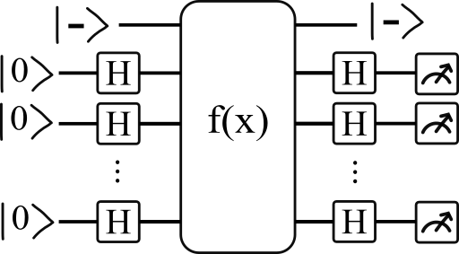
What can a quantum computer do with this oracle? It turns out that we can get the answer in exactly one query of the oracle. The circuit to do so is shown in Fig. 6
Three preliminary comments:
- As noted above, this is a phase oracle, so the input qubits will get a phase rotation depending on what the oracle’s response is. Generally, for an input bitstring in state $\ket{x}$, the output will look like $(-1)^{f(x)} * \ket{0}$. That is, a 180 degree phase will be applied to x if the oracle returns 1.
- There’s a new and unfamiliar block in the diagram, at the far right hand side of most of the qubits. That’s the symbol for measurement, and simply means we will measure each qubit (in the computational basis) and get $\ket{0}$ or $\ket{1}$ as possible results.
- You’ll notice the input qubits all go through a Hadamard gate before being fed into the oracle. Recall that a Hadamard gate moves qubits from the $\ket{0}$ to the $\ket{+}$ state. Recall further that a $\ket{+}$ state is an equal superposition between the $\ket{0}$ and $\ket{1}$ states. One way to think about this operation is that we are putting the set of n input qubits into an equal superposition of all possible bitstrings. If we were to measure the qubits after the first Hadamards but before the oracle, we have an equal chance of measuring every bitstring from $\ket{00..00}$ to $\ket{11..11}$. So we are thus applying the oracle to this state which represents the uniform superposition of all the input bitstrings.
I’m going to abstract away a lot of the details of the math in service of clarity, but we can express the state of the system before measurement as:
$$\frac{1}{\sqrt{2^N}} \sum_{x \in {0,1}^N} (-1)^{f(x)}H^{\otimes n} \ket{x}$$Where x is an individual N-length bitstring and $H^{\otimes n}$ is the Hadamard gate being applied to each of the n qubits. Expanding that second term over all the $n$ turns out to be non-trivial and produces an unwieldy expression. However, we can express the amplitude of the $\ket{00..00}$ state fairly simply:
$$ \alpha\ket{00..00} = \frac{1}{{2^N}} \sum_{x \in {0,1}^N} (-1)^{f(x)} \ket{00..00} $$Remember that $\alpha$, the amplitude of this state, represents the square root of the probability of measuring this state. Let’s evaluate this if $f(x)$ is constant: The argument of the summation always evaluates to 1 or -1 and there are $2^n$ different terms to evaluate, so the summation ends up being $2^n$ or $-2^n$. $\alpha$ is thus 1 or -1, and the probability of measuring the all-zero state is 1! This is an example of constructive interference, where amplitudes end up summing to increase the probability of a specific result.
If $f(x)$ is balanced, $f(x)$ will output 1 half the time and -1 the other half of the time, so the summation will evaluate to 0. The probability of measuring the all-zero state is thus 0. This is an example of destructive interference, where amplitudes end up canceling out to decrease the resulting probability of a state.
Operationally, the measurement occurs, and we can make an evaluation: If $\ket{00..00}$ is measured, we know that $f(x)$ is constant. If any other state is measured, $f(x)$ must be balanced. We’ve solved the problem in exactly 1 query to the oracle, substantially better than the classical case.
A few comments here:
- This is a very instructive demonstration of how quantum computing actually works. The popular media explanation of the field is: “Quantum computers will evaluate all possible inputs at once, then somehow report back the answer for a particular input”. This is not at all how this algorithm works. We put all possible inputs into the oracle via superposition, but rely on constructive and destructive interference to get the answer to the defined problem.
- Deutsch-Jozsa relies on an extremely specific problem statement with quite severe restrictions. This is what enables us to get the wonderful constructive/destructive interference results, and our $O(1)$ query complexity. Quantum computing theorists talk about the concept of ‘structure,’ which Deutsch-Jozsa is artificially designed to have. Put differently, certain problems simply have characteristics that make them amenable to being solved quantumly. Most people in the field think that for there to be a useful quantum speedup for a problem, there has to be at least some of this ‘structure’.
- Our quantum speedup is from a linear ($O(n)$) to a constant ($O(1)$) query complexity. This isn’t that good, and practically not enough to result in realistic quantum advantage for this contrived problem. Moreover, while the worst case bound on the classical case is ($n/2 + 1$) queries, if one is willing to accept a risk of error, one can get very high probability chance of success with even relatively small (~10 queries) amounts of classical queries, even for large values of n. Quantum algorithm designers are ‘at war’ with the classical algorithms – and the classical algorithms can fight back!
- We haven’t talked about how to implement the oracle. While the oracle is relatively simple in this case, it need not be. More on this when we discuss our next algorithm.
Models of Quantum Computation
Everything so far in this work has described computation through a lens of gate-based operations. The story I’m telling you is simple: start your qubits in an all $\ket{0}$ state, subject them to a bunch of gates, then measure at the end. This is often called the circuit-based model for quantum computing. This is not the only way to think about or implement quantum computation!
One well-known, but markedly different, model is adiabatic computation. Note first that the adiabatic model and the circuit (gate-based) model are proven to be mathematically identical. That is to say, anything you can do with gates, you can do adiabatically. Adiabatic computation is sort of an analog, more ‘physics-flavored’ way of implementing computations. The idea is that the qubits are prepared in a sort of initial state, and we are going to subject them to a time varying set of external fields (the physicists would call this a time-varying Hamiltonian). The ground state, or lowest energy state, of the initial Hamiltonian is equivalent to our initial prepared state. The ground state of the final Hamiltonian should be equivalent to the answer of the problem we want to solve. In the middle, the computer has to somehow interpolate between those two, perhaps linearly, although not necessarily.
This method might be a more natural and easier way of implementing certain algorithms or performing certain quantum physics simulations. In terms of commercial and academic interest, adiabatic methods seem to lag behind circuit-based computation. A notable exception is D-Wave Systems, which attempted to commercialize a technology that implemented ‘quantum annealing’. Quantum annealing was supposed to be a useful sub-set of a full adiabatic method, but appears to have produced no real effective results. D-Wave has recently acquired a superconducting qubit company, signaling that they, like most everyone else, are probably more thinking about gates and circuits than adiabatic computation.
Another notable alternative is ‘measurement-based’ quantum computation. Instead of subjecting qubits to a series of sequential operations, measurement-based computation generates what are called ‘cluster’ or ‘resource’ states, which are a large system of entangled qubits. The qubits are then progressively measured in specific ways that implement computation. The outcomes of initial measurements determine which qubits will be measured next, and how. This is also referred to as ‘one-way computation’, since the measurements cannot be reversed. This sort of approach is actually a very natural way of implementing computation for hardware that uses photons, for reasons we will discuss later.
In any case, it is helpful pedagogically to think about things in the circuit/gate-based model. It simply is easier to understand. Even the strange measurement based implementations typically start by taking an algorithm in circuit form, then compiling it to their measurement scheme.
Useful (?) Quantum Advantage: Grover’s Algorithm
We’ve now learned about a quantum algorithm that improves on any classical approach to the same problem. However, Deutsch-Jozsa’s algorithm applies to a totally trivial problem. We are now going to look at an algorithm with potentially broad applicability to a variety of tasks: Grover’s algorithm.
Grover’s algorithm was developed in 1996 by Lov Grover. Interestingly, Grover proposed this an algorithm for ‘database search’ problems. Unfortunately, the physical constraints of quantum computing make this a strange and impractical application of the approach. Grover’s is practically better suited for problems where the answer can be represented as the solution to an equation (this includes optimization problems), that is then made into the oracle.
Grover’s algorithm is a good deal more complex than Deutsch-Jozsa, and accordingly we will operate at a higher level of abstraction – thinking about operations rather than individual gates and states.
Let’s define the problem: We have a function $f(x)$, that takes in an n-bit value, and returns either 0 or 1. The function (or oracle) returns 1 for a particular value of x, and 0 otherwise. You can (as Grover did) conceive of this as a database search program – e.g. I have a phone number and I want to find the single owner of that phone number; or instead as some kind of math problem with a single optimal answer or condition that can be assessed by $f(x)$. In this way, Grover’s can be applied to extremely general problems if formulated correctly.
What’s the classical solution? Well, if we take the phone number example, we have to search through the phone book, line-by-line, until we find the match. This is called brute force searching, and is quite computationally expensive. For phone numbers of n-bits, this requires searching through on the order of $2^n$ entries. Thus, we would say it scales exponentially with $n$. To make notation simpler, we will call the total number of possible entries $N$ (which is equal to $2^n$). Note that for many problems, you can do better than this brute force search approach!
The quantum approach can do better than that. Before getting into the details, I’d like to introduce a very helpful mental model for thinking about this problem. Let’s say we have n qubits. At the end of our computation, we will measure those qubits and they will be in one of $N=2^n$ states, just like how n bits can represent $2^n$ different values. In the middle of computation, the qubits will be in some intermediate state, which can be expressed as a linear combination of several or all of those N states. We can represent this intermediate state via a N dimensional vector, as shown below for a 4-qubit example:
$$\left[ \begin{matrix} \sqrt{P(\ket{0000})} \\ \sqrt{P(\ket{0010})} \\ \sqrt{P(\ket{0011})} \\ \vdots \\ \sqrt{P(\ket{1111})} \\ \end{matrix} \right] $$Unfortunately, it’s difficult to visualize that vector. If it were 2- or 3-dimensions, we could graph it, but as a species living in 3-dimensions, it’s pretty tricky for us humans to imagine $2^4 = 16$-dimensional vector spaces in our mind. What we can do though, is compress this higher-dimensional vector space into 2 dimensions. Remember that every single dimension, or row, of this vector simply corresponds to a different output state of the set of qubits. When we look at the value in the vector in a particular dimension, we are just evaluating the probability of the qubits being measured in that state. Thus, the two effective dimensions we will pick (for the purpose of understanding Grover’s algorithm) are: 1) the dimension that corresponds to the correct solution to our search problem; 2) all the other ones combined – i.e. the wrong answers. This will hopefully become clearer in a moment.
We’re going to begin in the same way we did in Deutsch-Jozsa: Feeding n $\ket{0}$ state initialized qubits into a set of Hadamard gates. As we noted before, the qubits are now in an equal superposition between the $N=2^n$ possible output bitstrings. How should this look in our 2-D representation? Well, if we were to measure the qubits now, our probability of getting the correct answer would be 1/N – it’s totally random chance. Thus, there will only be some small component of the vector space that points toward the correct answer, and the dimension that contains every other answer will be much larger. We draw this in Fig. 7. $\ket{t}$ represents the ‘noT right’ answers; $\ket{r}$ the ‘Right’ answer; and $\ket{e}$ the ‘Equal everything’ vector.
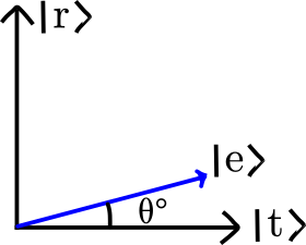
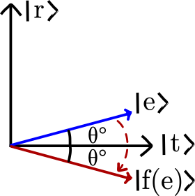
Note that theta – the angle that $\ket{e}$ deviates from $\ket{t}$ - will be smaller the larger $n$ is. The next step is to feed our qubits into our oracle. Just like in Deutsch-Jozsa, we’re going to use a phase oracle. The sign of the correct answer will be inverted, but otherwise the qubits will stay in the same state. This is equivalent to reflecting our qubits around the ‘not-right’ axis. This is easy to visualize, and shown in Fig. 8.
Here’s the most conceptually tricky step: We need to reflect our qubits around that initial, equal superposition state. I’m not going to explain how to do this. You really don’t care do you? Just know: We can do this. If you really care, read a textbook*. Now what state are our qubits in? Look at Fig. 9.
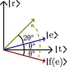
Notice that we are now closer to the ‘right answer’ axis! If we measured the qubits now, we would be more likely to measure the correct answer than when we started. Wow! Unfortunately, that probability still could be small, depending on how big n is (and thus, how small $\theta$ is). Our solution is to simply repeat this process again and again: First we use the oracle and reflect across ‘not-the-answer’, then reflect across the ‘equal-superposition’ state to get closer to pointing toward ‘the-answer’. To get the vector pointing towards ‘the-answer’ we repeat this process $\sqrt{N}$ times, as shown in Fig. 10. We can then measure the qubits and get the correct answer with very high probability! We’ve beaten the classical approach by a factor of $\sqrt{N}$!
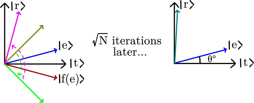
This sqrt(N) speedup is often called a ‘quadratic’ or ‘Grover’ speedup and is commonly found in many quantum algorithms. In some ways, this is excellent: For large values of n, this might be a huge reduction in oracle queries necessary to find the solution. It’s also just sort of magical that via superposition and quantum-ness, we can somehow parse through $2^n$ possible entries in way fewer queries. But in other ways, it is not so exciting: Problems that take exponential time (‘NP Hard’ problems) still take exponential time, because $O(2^n/\sqrt{2^n})$ is still exponential complexity. As discussed previously, physical implementations of quantum computers are expected to run at slower clock frequencies than classical computers, so a quadratic quantum speedup may still be slower than a classical approach. And importantly, it might be really hard to implement that oracle! This is the fatal flaw with using Grover’s for database search. We need an oracle that somehow ‘knows’ which answer is correct, despite that being the problem we are trying to solve! In classical computing, that oracle would be implemented via querying some sort of structured memory where our database lives. Unfortunately, implementing a ‘quantum memory’ (often referred to as a quantum RAM, for random access memory), where we can query lots of data in superposition, is extremely difficult, and perhaps impossible,* making Grover’s even more difficult to implement.
Where does this leave us? Grover’s is extremely cool and a useful tool in the proverbial toolbox, but unlikely to be the foundation of quantum’s ‘killer app’. Onwards we go…
No Cloning
I’ve mentioned above that it’s difficult, perhaps impossible, to make a quantum memory. One reason for this is the ‘no-cloning theorem’. We’d like to make a copy of some data to put into our theoretical memory, like so:
$$\ket{\psi}\ket{0} \rightarrow \ket{\psi}\ket{\psi}$$It turns out, that for unknown $\ket{\psi}$, this is not possible! There is no generic quantum gate that enables us to duplicate our qubits. This makes certain algorithms more difficult to implement, and makes error correction MUCH harder (more on that later). More generally, it challenges our ability to think of quantum computers as simply quantum versions of regular computers. It is so critical for a normal CPU’s operation to reach into memory to pull out certain values, or to put results into memory. This is not a trivial operation in the quantum world.
Useful Quantum Advantage: Shor’s Algorithm
Now we turn our attention to Shor’s algorithm – the most famous (and potentially most useful) quantum algorithm. Invented by Peter Shor in 1993, Shor’s algorithm is a method of factoring large numbers. Factoring is a very important problem, since most modern encryption schemes rely on factoring being hard in order to guarantee security. RSA (named after its inventors, Rivest, Shamir, & Adleman), one of the most widely used encryption schemes, uses two large prime numbers to generate both a public and private key. If one could factorize the public key, it would be trivial to generate the private key and thus be able to decrypt the secret data.
Fortunately, factoring is classically difficult. The best-known classical algorithm, called the general number field sieve, scales with approximately $O(e^{n^{1/3})}$, which is sub-exponential but not efficient. Thus, our cryptographic schemes are currently secure! But quantum computers should be able to do better, utilizing Shor’s algorithm. We will again examine this algorithm with a bit more abstraction, looking at the steps taken rather than the individual gates. Shor’s algorithm takes a number N which is the product of two large primes, p and q. N is known, but we would like to find p and q.
- We pick a number $a$ in between 1 and N. We check if it is a factor or a multiple of a factor of $N$ (i.e. did we luck into picking the right answer). If it is, we succeeded! If it isn’t, we move onto step 2. Note that this is a classical computation, not a quantum one.
- This is the fantastic quantum-accelerated step. We perform an operation called ‘period finding’ using a and N. The operation $a^x$ modulo $N$ has a property where as values of x are stepped through, the modulus will end up cycling through a set of values. We can find out the length of the cycle, known as a period, with a period finding algorithm. This operation, performed quantumly, has complexity $O(n^3)$, which is polynomial and thus efficient! It produces the period, r.
- We now have a and r. It turns out that $a^{(r/2)}+1$ and $a^{(r/2)}-1$ have a wonderful property, which is that they each share a common factor with N. Thus, we just figure out the greatest common denominator between those terms and $N$, and we have p and q respectively. Again, note that this is a classical step.
Shor’s thus can factor large numbers in polynomial time, significantly better than any known classical approach. This obviously has large potential impacts on digital information security, but we will reserve discussing those implications for Section III: Applications.
I do want to note a few things specifically about Shor’s as an algorithm here:
- Shor’s is, to our knowledge, the only quantum algorithm that is practically useful and has a provable exponential speedup over known classical approaches. It is, without exaggeration, the bedrock which the field’s current level of funding and interest lies upon. As such, there is considerable interest in using Shor’s as a sort of benchmark – i.e. how large of a number can you factor on your quantum computer using Shor’s? Unfortunately, factoring even small numbers requires a large amount of quantum computational resources: This excellent Craig Gidney (a prolific researcher at Google Quantum AI*) article estimates that factoring the number 21 requires approximately 2,400 multi-qubit gates. That’s a lot! As such, there’s a small cottage industry of researchers and institutions using numerical tricks to ‘factor’ large numbers ‘quantumly’. The only upside of this is the delightful tiny cottage industry of researchers debunking or skewering these factorizations, which reached its apex with: “Replication of Quantum Factorisation Records with an 8-bit Home Computer, an Abacus, and a Dog.”
- It is explicitly a classical/quantum hybrid algorithm. It specifically uses the quantum computer to perform a subroutine which is (relatively) easy quantumly, but hard classically. In general, we want to do as little as possible on the quantum side, leveraging our classical infrastructure as much as possible. This will be true for many of the potential applications of quantum computing we will discuss later in this work.
- Remember how we discussed that the ‘structure’ of the problem poised in Deutsch-Jozsa was what enabled the quantum speedup? In the same way, Shor’s exploits the ‘structure’ of the problem. Factoring large numbers (and specifically period finding) has some specific relation to the ‘hidden subgroup problem’ for finite Abelian groups*. It’s plausible that other problems may relate to this hidden subgroup concept in some way, and thus a Shor’s-level speedup may be accessible in such cases. Unfortunately, those problems haven’t yet been found.
Commentary
If you’ve followed thus far, you now understand how quantum computation differs from classical computation and how it can speed up the calculation of certain problems. This is roughly what you would get from an elementary quantum information and computation textbook, albeit with much less rigor. Perhaps it answers a base curiosity about what quantum computation is. Perhaps it sparks even more questions, about how these mathematical objects can be implemented in real life, and if those quantum algorithms can perform useful calculations outside of academic proposals. If so, please read on.
References
- William Kretschmer et al., Demonstrating an unconditional separation between quantum and classical information resources, Version Number: 2, 2025, accessed June 18, 2026, https://doi. org/10.48550/ARXIV.2509.07255, https://arxiv.org/abs/2509.07255.
- A. Holevo, “Bounds for the quantity of information transmitted by a quantum communication channel” (1973), accessed June 18, 2026, https://www.semanticscholar.org/paper/Bounds- for-the-quantity-of-information-transmitted-Holevo/0733393a545b62e49e9fc4a76d53d843cf b72010.
- Ehud Altman et al., “Quantum Simulators: Architectures and Opportunities,” PRX Quantum 2, no. 1 (February 24, 2021): 017003, issn: 2691-3399, accessed November 20, 2025, https: //doi.org/10.1103/PRXQuantum.2.017003, https://link.aps.org/doi/10.1103/PRXQuantum. 2.017003.
- David Deutsch and Richard Jozsa, “Rapid Solution of Problems by Quantum Computation,” Proceedings: Mathematical and Physical Sciences 439, no. 1907 (1992): 553–558, issn: 0962- 8444, accessed June 18, 2026, https://www.jstor.org/stable/52182.
- Dorit Aharonov and Wim van Dam, “Adiabatic Quantum Computation is Equivalent to Standard Quantum Computation.”
- Lov K. Grover, A fast quantum mechanical algorithm for database search, arXiv:quant-ph/9605043, November 19, 1996, accessed April 19, 2026, https://doi.org/10.48550/arXiv.quant-ph/9605043, arXiv: quant-ph/9605043, http://arxiv.org/abs/quant-ph/9605043.
- W. K. Wootters and W. H. Zurek, “A single quantum cannot be cloned,” ADS Bibcode: 1982Natur.299..802W, Nature 299 (October 1, 1982): 802–803, issn: 0028-0836, accessed May 6, 2026, https://doi.org/10.1038/299802a0, https://ui.adsabs.harvard.edu/abs/1982Natur.299. .802W.
- Peter W. Shor, “Polynomial-Time Algorithms for Prime Factorization and Discrete Logarithms on a Quantum Computer,” SIAM Journal on Computing 26, no. 5 (October 1997): 1484–1509, issn: 0097-5397, 1095-7111, accessed June 17, 2026, https://doi.org/10.1137/S0097539795293 172, arXiv: quant-ph/9508027, http://arxiv.org/abs/quant-ph/9508027.
- Peter Gutmann and Stephan Neuhaus, “Replication of Quantum Factorisation Records with an 8-bit Home Computer, an Abacus, and a Dog.”